Excel – Power query

Over the last few years, our department at work have been looking at ways we can improve efficiency.

As with many other finance departments our work is dominated by Excel. With quite a lot of repetitive tasks being undertaken in Excel. Power Query has literally changed how we approach a lot of tasks within Excel. However the leap over to using this fantastic tool took some additional steps to get working.

Power Query for Finance Teams

There are a few tutorials on how to get started with Power Query, but below is a practical example that you will be able to get started with right away.

Let’s start with an easy example. Imagine you have a dataset of regional sales by product, in your usual report you add a formula – probably a vlookup or an xlookup to bring through the product category.

We can use Power Query to automate the vlookup process so we never have to do it again!

Step 1 – Download the Workbook & Follow Along!

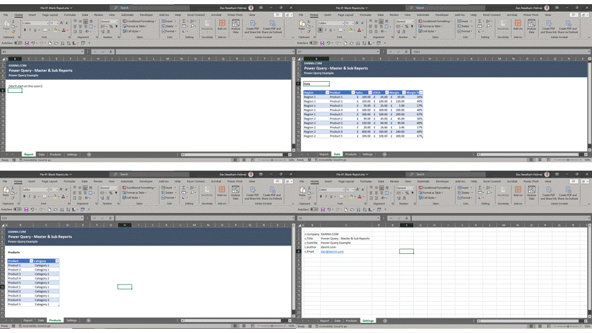
We’ll be starting with the following tabs:

1. Report tab – this will come later!
2. Data – our sales report
3. Product List – Lookup for categories
4. Settings – constants for the workbook and checks – we’ll visit this another time

Loading Our Data into Power Query

Report Data

• Starting on the Data tab, click anywhere in the data table.
• On the top menu bars, click “Data”, under the get and transform section, click “From Table/Range”
• Click on close and load to, select table then OK.
• On the next popup, click on the Existing Worksheet Option
• Click the arrow, then select the Report tab, and select any cell to place your Power Query table.
  

Lookup Data

We’ll repeat most of the steps above for our product lookup table.

• Go to the product tab, select anywhere within the data table.
• Click “Data”, then “From Table/Range”
• Click close and load to, but this time, select “Only create connection” and click OK.

Wait, nothing happened! The magic happens next!

Automate That VLookup!

There have been quite a few steps to this point. This tutorial is about automating repetitive tasks, this isn’t designed as a replacement for vlookups. This is more for speeding up a regular report. The time taken now will be saved in future!

To get back into Power Query, select the data menu, click “Get Data”, then click “Launch Power Query Editor”.

We’re going to use a function called merging. This allows us to join data from another table that we’ve already loaded into Power Query.

• Select the Data table on the left hand menu.
• Under the combine section on the top menu, click “Merge Queries”.
• The window that pops up has the data table at the top, select the product table in the drop down.
• Now highlight the product in both tables by clicking on them, they should highlight in blue.
• Click ok.
• Re-order the columns as needed. I’ve moved the category before the product ID.
• Click close and load.
  

That’s it, our data now includes the category information! This can now be your base report that you can use every time you update this information. No need to re-do any of the steps above, just drop your data into the data tab!

To refresh the report data, head to data and click “Refresh All” your report data will refresh automatically!

Check out the next article (Error Checking is Key) for the obvious mistake and why error checking is so important!